I’ve spent a lot of time lately on homelab topics, so I thought I would take a break and put together a post on an EPM topic! Today we’ll be talking about PBCS backups.
Why Do We Need PBCS Backups
You might be thinking, “Why do I need PBCS backups when Oracle does that for me?” That’s an excellent question. The problem is that while Oracle does perform nightly backups of PBCS, they overwrite that backup each night. So at any given time I only have one backup. To make things even worse, Oracle has a size limit on your PBCS instance. That limit is 150GB. This means that even if we had multiple backups on our pod, we’ll eventually start losing them to the data retention policies.
So what do we do? We generate a new backup every night and download it to a local server. The good news is that you almost certainly have a local server already running EPM Automate. EPM Automate is the automation tool for Oracle’s EPM Cloud suite. You can use EPM Automate to load data, execute calculations, update meta-data, and…perform backups. So, we’ve established that we likely need more than a single night of backups, but how many do we need? This will depend on a few things like the size of your applications and the frequency of change. For our example, we will keep 30 days of daily backups.
Batch vs. PowerShell
Now that we have determined what we are backing up and how many backups we need to keep, we need to move on to actually performing the backups. With EPM Automate, we have two commonly used options. First, we have the old-school method of a batch file. Batch files are great because they just work and you can find a ton of information on the web about how to do things. Batch are, however, very limited in their ability to do things like e-mail notifications and remote calls without external tools. That brings us to PowerShell. PowerShell is essentially a batch that has the full set of .NET programming capability along with other goodies not directly from .NET. What does that mean exactly? That means there is very little I can’t do in PowerShell.
Directory Configuration
Before we configure anything, we need to get a folder structure put together to support scripting, logging, and the actual backup files. You may already have a structure for your automation processes, but for our example, it will look something like this:
- C:\Oracle
- C:\Oracle\Automation
- C:\Oracle\Automation\Backup
- C:\Oracle\Automation\Log
- C:\Oracle\Automation
EPM Automate Configuration
EPM Automate is a great tool, but we do need to perform a little bit of setup to get going. For instance, while EPM Automate supports plain text passwords, that wouldn’t pass muster with most IT security groups. So before we get into PowerShell, let’s encrypt our password. This is a fairly easy process. We’ll start up a command prompt and change directory to our EPM Automate bin directory:
cd\
cd Oracle\EPM_Automate\bin
Once we are in the right directory, we can encrypt our password:
epmautomate.bat encrypt YourPasswordGoesHere PickYourKey c:\Oracle\Automation\password.epw
Here are the parameters:
- Command – the command EPM Automate will execute
- encrypt
- Password – the password of the account you plan to use
- YourPasswordGoesHere
- Key – you specify anything you want to use to encrypt the password
- PickYourKey
- Password File – The full path and file name of the password file that will be generated
- c:\Oracle\Automation\password.epw
Once we execute the command, we should have our password file so that we can continue. It should look something like this:

Backing Up PBCS with PowerShell
For our first part of this mini-series, we’ll stick with just a basic backup that deletes older backups. In our next part of the series, we’ll go deeper into error handling and notifications. Here’s the code..
Path Variables
#Path Variables
$EpmAutomatePath = "C:\Oracle\EPM_Automate\bin\epmautomate.bat"
$AutomationPath = "C:\Oracle\Automation"
$LogPath = "C:\Oracle\Automation\Log"
$BackupPath = "C:\Oracle\Automation\Backup"
We’ll start by defining our path variables. This will include paths to EPM Automate, our main automation directory, our log path, and our backup path.
Date Variables
#Date Variables
$DaysToKeep = "-30"
$CurrentDate = Get-Date
$DatetoDelete = $CurrentDate.AddDays($DaysToKeep)
$TimeStamp = Get-Date -format "yyyyMMddHHmm"
$LogFileName = "Backup" + $TimeStamp + ".log"
Next we’ll define all of our data related variables. This includes our days to keep (which is negative on purpose as we are going back in time), our current date, the math that gets us back to our deletion period, a timestamp that will be used for various things, and finally our log file name based on that timestamp.
PBCS Variables
#PBCS Variables
$PBCSdomain = "yourdomain"
$PBCSurl = "https://usaadmin-test-yourdomain.pbcs.us2.oraclecloud.com"
$PBCSuser = "yourusername"
$PBCSpass = "c:\Oracle\Automation\password.epw"
Now we need to set our PBCS variables. This will include our domain, the URL to our instance of PBCS, the username we’ll use to log in, and the path to the password file that we just finished generating.
Snapshot Variables
#Snapshot Variables
$PBCSExportName = "Artifact Snapshot"
$PBCSExportDownloadName = $PBCSExportName + ".zip"
$PBCSExportRename = $PBCSExportName + $TimeStamp + ".zip"
We’re nearing the end of variables as we define our snapshot specific variables. These variables will tell us the name of our export, the name of the file that we are downloading based on that name, and the new name of our snapshot that will include our timestamp.
Start Logging
#Start Logging
Start-Transcript -path $LogPath\$LogFileName
I like to log everything so that if something does go wrong, we have a chance to figure it out after the fact. This uses the combination of our log path and log file name variables.
Log Into PBCS
#Log into PBCS
Write-Host ([System.String]::Format("Login to source: {0}", [System.DateTime]::Now))
&$EpmAutomatePath "login" $PBCSuser $PBCSpass $PBCSurl $PBCSdomain
We can finally log into PBCS! We’ll start by displaying our action and the current system time. This way we can see how long things take when we look at the log file. We’ll then issue the login command using all of our variables.
Create the Snapshot
#Create PBCS snapshot
Write-Host ([System.String]::Format("Export snapshot from source: {0}", [System.DateTime]::Now))
&$EpmAutomatePath exportsnapshot $PBCSExportName
Again we’ll display our action and current system time. We then kick off the snapshot process. We do this because we want to ensure that we have the most recent snapshot for our archiving purposes.
Download the Snapshot
#Download PBCS snapshot
Write-Host ([System.String]::Format("Download snapshot from source: {0}", [System.DateTime]::Now))
&$EpmAutomatePath downloadfile $PBCSExportName
Once the snapshot has been created, we’ll move on to downloading the snapshot after we display our action and current system time.
Archive the Snapshot
#Rename the file using the timestamp and move the file to the backup path
Write-Host ([System.String]::Format("Rename downloaded file: {0}", [System.DateTime]::Now))
Move-Item $AutomationPath\$PBCSExportDownloadName $BackupPath\$PBCSExportRename
Once the file has been downloaded, we can then archive the snapshot to our backup folder as we rename the file.
Delete Old Snapshots
#Delete snapshots older than $DaysToKeep
Write-Host ([System.String]::Format("Delete old snapshots: {0}", [System.DateTime]::Now))
Get-ChildItem $BackupPath -Recurse | Where-Object { $_.LastWriteTime -lt $DatetoDelete } | Remove-Item
Now that we have everything archived, we just need to delete anything older than our DateToDelete variable.
Log Out of PBCS
#Log out of PBCS
Write-Host ([System.String]::Format("Logout of source: {0}", [System.DateTime]::Now))
&$EpmAutomatePath "logout"
We’re almost done and we can now log out of PBCS.
Stop Logging
#Stop Logging
Stop-Transcript
Now that we have completed our process, we’ll stop logging
The Whole Shebang
#Path Variables
$EpmAutomatePath = "C:\Oracle\EPM_Automate\bin\epmautomate.bat"
$AutomationPath = "C:\Oracle\Automation"
$LogPath = "C:\Oracle\Automation\Log"
$BackupPath = "C:\Oracle\Automation\Backup"

#Date Variables
$DaysToKeep = "-30"
$CurrentDate = Get-Date
$DatetoDelete = $CurrentDate.AddDays($DaysToKeep)
$TimeStamp = Get-Date -format "yyyyMMddHHmm"
$LogFileName = "Backup" + $TimeStamp + ".log"

#PBCS Variables
$PBCSdomain = "yourdomain"
$PBCSurl = "https://usaadmin-test-yourdomain.pbcs.us2.oraclecloud.com"
$PBCSuser = "yourusername"
$PBCSpass = "c:\Oracle\Automation\password.epw"

#Snapshot Variables
$PBCSExportName = "Artifact Snapshot"
$PBCSExportDownloadName = $PBCSExportName + ".zip"
$PBCSExportRename = $PBCSExportName + $TimeStamp + ".zip"

#Start Logging
Start-Transcript -path $LogPath\$LogFileName

#Log into PBCS
Write-Host ([System.String]::Format("Login to source: {0}", [System.DateTime]::Now))
&$EpmAutomatePath "login" $PBCSuser $PBCSpass $PBCSurl $PBCSdomain

#Create PBCS snapshot
Write-Host ([System.String]::Format("Export snapshot from source: {0}", [System.DateTime]::Now))
&$EpmAutomatePath exportsnapshot $PBCSExportName

#Download PBCS snapshot
Write-Host ([System.String]::Format("Download snapshot from source: {0}", [System.DateTime]::Now))
&$EpmAutomatePath downloadfile $PBCSExportName

#Rename the file using the timestamp and move the file to the backup path
Write-Host ([System.String]::Format("Rename downloaded file: {0}", [System.DateTime]::Now))
Move-Item $AutomationPath\$PBCSExportDownloadName $BackupPath\$PBCSExportRename

#Delete snapshots older than $DaysToKeep
Write-Host ([System.String]::Format("Delete old snapshots: {0}", [System.DateTime]::Now))
Get-ChildItem $BackupPath -Recurse | Where-Object { $_.LastWriteTime -lt $DatetoDelete } | Remove-Item

#Log out of PBCS
Write-Host ([System.String]::Format("Logout of source: {0}", [System.DateTime]::Now))
&$EpmAutomatePath "logout"

#Stop Logging
Stop-Transcript
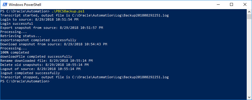
The Results
Once you execute the PowerShell script, you should see something like this:
Conclusion
There we have it…a full process for backing up your PBCS instance. The last step would be to set up a scheduled task to execute once a day avoiding your maintenance window.