Welcome to the seventh part in an on-going blog series about Essbase performance. Today we will focus on Essbase Physical vs. Virtual Performance, but first here’s a summary of the series so far:
- Essbase Performance Series: Part 1 – Introduction
- Essbase Performance Series: Part 2 – Local Storage Baseline (CDM)
- Essbase Performance Series: Part 3 – Local Storage Baseline (Anvil)
- Essbase Performance Series: Part 4 – Network Storage Baseline (CDM)
- Essbase Performance Series: Part 5 – Network Storage (Anvil)
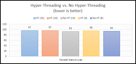
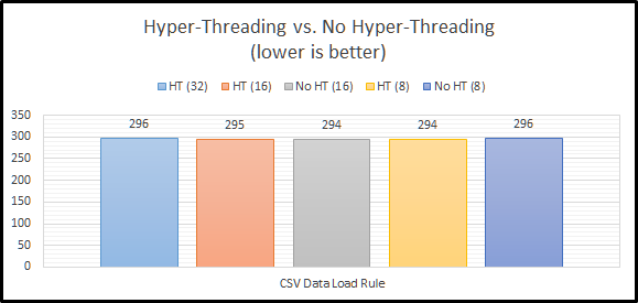
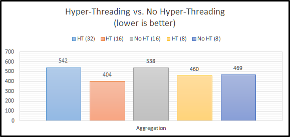
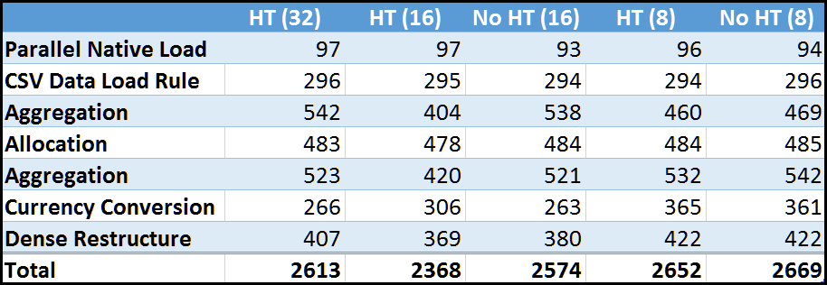
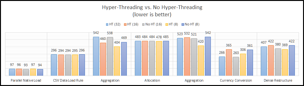
- Essbase Performance Series: Part 6 – Essbase and Hyper-Threading
- Essbase Performance Series: Part 7 – Physical vs. Virtual – Native Loads
I started sharing actual Essbase benchmark results in part six of this series, focusing on Hyper-Threading. Today I’ll shift gears away from physical Essbase testing and focus on virtualized Essbase.
Testing Configuration
All testing is performed on a dedicated benchmarking server. This server changes software configurations between Windows and ESXi, but the hardware configuration is static. Here is the physical configuration of the server:
| Processor(s) | (2) Intel Xeon E5-2670 @ 2.6 GHz |
| Motherboard | ASRock EP2C602-4L/D16 |
| Memory | 128 GB - (16) Crucial 8 GB ECC Registered DDR3 @ 1600 MHz |
| Chassis | Supermicro CSE-846E16-R1200B |
| RAID Controller | LSI MegaRAID Internal SAS 9265-8i |
| Solid State Storage | (4) Samsung 850 EVO 250 GB on LSI SAS in RAID 0 |
| Solid State Storage | (2) Samsung 850 EVO 250 GB on Intel SATA |
| Solid State Storage | (1) Samsung 850 EVO 250 GB on LSI SAS |
| NVMe Storage | (1) Intel P3605 1.6TB AIC |
| Hard Drive Storage | (12) Fujitsu MBA3300RC 300GB 15000 RPM on LSI SAS in RAID 10 |
| Network Adapter | Intel X520-DA2 Dual Port 10 Gbps Network Adapter |
I partitioned each of the storage devices into equal halves: one half for use in the Windows installation on the physical hardware and one half for use in the VMware ESXi installation. here is the virtual configuration of the server:
| Processors | 32 vCPU (Intel Xeon E5-2670) |
| Memory | 96GB RAM (DDR3 1600) |
| Solid State Storage | (4) Samsung 850 EVO 250 GB on LSI SAS in RAID 0 (Data store) |
| Solid State Storage | (1) Samsung 850 EVO 250 GB on LSI SAS (Data store) |
| NVMe Storage | Intel P3605 1.6TB AIC (Data store) |
| Hard Drive Storage | (12) Fujitsu MBA3300RC 300GB 15000 RPM on LSI SAS in RAID 10 (Data store) |
| Network Adapter | Intel X520-DA2 Dual Port 10 Gbps Network Adapter |
Network Storage
Before we get too far into the benchmarks, I should probably also talk about iSCSI and network storage. iSCSI is one of the many options out there to provide network-based storage to servers. This is one implementation used by many enterprise storage area networks (SAN). I implemented my own network attache storage device so that I could test out this type of storage. Network storage is even more common today because most virtual clusters require some sort of network storage to provide fault tolerance. Essentially, you have one storage array that is shared by multiple hosts. This simplifies back-ups and maintains high availability and performance.
There is however a problem. Essbase is heavily dependent on disk performance. Latency of any kind will harm performance because as latency increases, random I/O performance decreases. So why does network storage have a higher latency? Let’s take a look at our options.
Physical Server with Local Storage
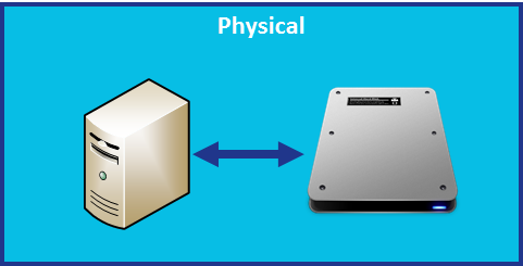
In this configuration, the disk is attached to the physical server and the latency is contained inside of the system. Think of it like a train: the longer we travel on a track, the longer it takes to reach out destination and return home.
Virtual Server with Local Storage
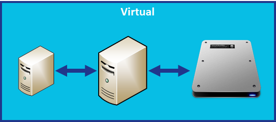
With virtual storage, we have a guest server that communicates to the host server for I/O requests that has a disk attached. Now our train is traveling on a little bit more track. So latency increases and performance decreases.
Physical Server with Network Storage
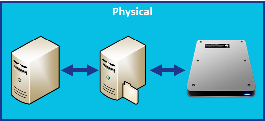
Our train track seems to be getting longer by the minute. With network storage on a physical server, we now have our physical server communicating with our file server that has a disk attached. This adds an additional stop.
Virtual Server with Network Storage
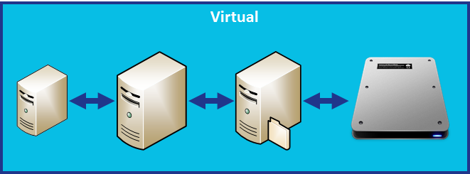
This doesn’t look promising at all. Our train now makes a pretty long round-trip to reach its destination. So performance might not be great on this option for Essbase. That’s unfortunate, as this is a very common configuration. Let’s see what happens.
EssBench Application
The application used for all testing is EssBench. This application has the following characteristics:
- Dimensions
- Account (1025 members, 838 stored)
- Period (19 members, 14 stored)
- Years (6 members)
- Scenario (3 members)
- Version (4 members)
- Currency (3 members)
- Entity (8767 members, 8709 stored)
- Product (8639 members, 8639 stored)
- Data
- 8 Text files in native Essbase load format
- 1 Text file in comma separated format
- PowerShell Scripts
- Creates Log File
- Executes MaxL Commands
- MaxL Scripts
- Resets the cube
- Loads data (several rules)
- Aggs the cube
- Executes allocation
- Aggs the allocated data
- Executes currency conversion
- Restructures the database
- Executes the MaxL script three times
Testing Methodology
For these benchmarks to be meaningful, we need to be consistent in the way that they are executed. The tests in both the physical and virtual environment were kept exactly the same on an Essbase level. Today I will be focusing on native Essbase loads. The process takes eight (8) native Essbase files produced from a parallel export and loads them into Essbase using a parallel import. Because this is a test of loading data, CALCPARALLEL and RESTRUCTURETHREADS have no impact. Let’s take a look at the steps used to perform these tests:
- Physical Test – Intel P3605
- A new instance of EssBench was configured using the application name EssBch06.
- The data storage was changed to the Intel P3605 drive.
- The application was restarted.
- The EssBench process was run for this instance and the results collected. The three sets of results were averaged and put into the chart and graph below.
- Physical Test – SSD RAID
- A new instance of EssBench was configured using the application name EssBch08.
- The data storage was changed to the SSD RAID drive.
- The application was restarted.
- The EssBench process was run for this instance and the results collected. The three sets of results were averaged and put into the chart and graph below.
- Physical Test – Single SSD
- A new instance of EssBench was configured using the application name EssBch09.
- The data storage was changed to the single SSD drive.
- The application was restarted.
- The EssBench process was run for this instance and the results collected. The three sets of results were averaged and put into the chart and graph below.
- Physical Test – iSCSI NVMe
- A new instance of EssBench was configured using the application name EssBch10.
- The data storage was changed to the iSCSI NVMe drive.
- The application was restarted.
- The EssBench process was run for this instance and the results collected. The three sets of results were averaged and put into the chart and graph below.
- Physical Test – iSCSI HDD w/ SSD Cache
- A new instance of EssBench was configured using the application name EssBch11.
- The data storage was changed to the iSCSI HDD drive.
- The application was restarted.
- The EssBench process was run for this instance and the results collected. The three sets of results were averaged and put into the chart and graph below.
- Physical Test – HDD RAID
- A new instance of EssBench was configured using the application name EssBch07.
- The data storage was changed to the HDD RAID drive.
- The application was restarted.
- The EssBench process was run for this instance and the results collected. The three sets of results were averaged and put into the chart and graph below.
- Virtual Test – Intel P3605
- A new instance of EssBench was configured using the application name EssBch15.
- The data storage was changed to the Intel P3605 drive.
- The application was restarted.
- The EssBench process was run for this instance and the results collected. The three sets of results were averaged and put into the chart and graph below.
- Virtual Test – SSD RAID
- A new instance of EssBench was configured using the application name EssBch16.
- The data storage was changed to the SSD RAID drive.
- The application was restarted.
- The EssBench process was run for this instance and the results collected. The three sets of results were averaged and put into the chart and graph below.
- Virtual Test – Single SSD
- A new instance of EssBench was configured using the application name EssBch17.
- The data storage was changed to the single SSD drive.
- The application was restarted.
- The EssBench process was run for this instance and the results collected. The three sets of results were averaged and put into the chart and graph below.
- Virtual Test – iSCSI NVMe
- A new instance of EssBench was configured using the application name EssBch18.
- The data storage was changed to the iSCSI NVMe drive.
- The application was restarted.
- The EssBench process was run for this instance and the results collected. The three sets of results were averaged and put into the chart and graph below.
- Virtual Test – iSCSI HDD w/ SSD Cache
- A new instance of EssBench was configured using the application name EssBch19.
- The data storage was changed to the iSCSI HDD drive.
- The application was restarted.
- The EssBench process was run for this instance and the results collected. The three sets of results were averaged and put into the chart and graph below.
- Virtual Test – HDD RAID
- A new instance of EssBench was configured using the application name EssBch14.
- The data storage was changed to the HDD RAID drive.
- The application was restarted.
- The EssBench process was run for this instance and the results collected. The three sets of results were averaged and put into the chart and graph below.
So…that was a lot of testing. Luckily, that set of steps will apply to the next several blog posts.
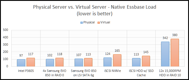
Physical vs. Virtual Test Results
This is a very simple test. It really just needs a disk drive that can provide adequate sequential writes, and things should be pretty fast. So how did things end up? Let’s break it down by storage type.
Intel P3605
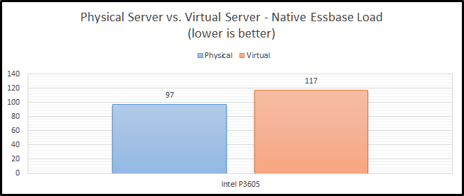
The Intel P3605 is an enterprise-class NVMe PCIe SSD. Beyond all of the acronyms, its basically a super-fast SSD. When comparing these two configurations, we see that clearly the physical server is much faster (21%).
SSD RAID

I’ve chosen to implement SSD RAID using a physical LSI 9265-8i SAS controller with 1GB of RAM. The drives are configured in RAID 0 to get the most performance possible. RAID 1+0 is preferred, but then I would need eight drives to get the same performance level. The finance committee (my wife) would frown on another four drives. Our SSD RAID option is still faster on a physical server, as we would expect. The difference however is lower at 16%. It is also worth noting that it is basically the same speed as our NVMe option in the virtual configuration. I believe this is likely due to the drivers for Windows being better for the NVMe SSD than they are for ESXi.
Single SSD
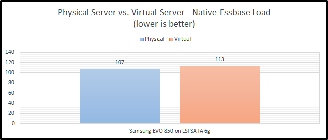
How did our single SSD fair? Pretty well actually with only a 5% decrease in performance going to a virtual environment. In our virtual environment, we actually see that it is faster than both our NVMe and SSD RAID options. But…they are pretty close. We’ll wait to see how everything performs in later blog posts before we draw any large conclusions from this test.
iSCSI NVMe
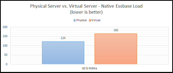
Now we can move on to a little bit more interesting set of benchmarks. Network storage never seems to work out at my clients. It especially seems to struggle as they go virtual. Here, we see that NVMe over iSCSI performs “okay” on a physical system, but not so great on a virtual platform. The difference is a staggering 34%.
iSCSI HDD w/ SSD Cache
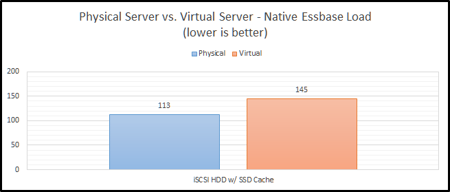
Staying on the topic of network storage, I also tested out a configuration with hard drives and an SSD cache. The problem with this test is that I’m the only user on the system and the cache is a combination of 200GB of SSD and a ton of RAM. Between those two things, I don’t think it ever leaves the cache. The difference between physical and virtual is still pretty bad at 28%. I still can’t explain why this configuration is faster than the NVMe configuration, but my current guess is that it is related to drivers and/or firmware in FreeBSD.
HDD RAID
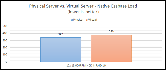
Finally, we come to our slowest option…old-school hard drives. It isn’t just a little slower…it is a LOT slower. This actually uses the same RAID card that I am using for the SSD RAID configuration. These drives are configured in RAID 1+0. With the SSD’s, I was trying to see how fast I can make it. With the HDD configuration, I was really trying to test out a real-world configuration. RAID 0 has no redundancy, so it is very uncommon with hard drives. We see here that the hard drive configuration is only 11% slower in a virtual configuration than in a physical configuration. We’ll call that the silver lining.
Summarized Essbase Physical vs. Virtual Performance Results
Let’s look at the all of the results in a grid:
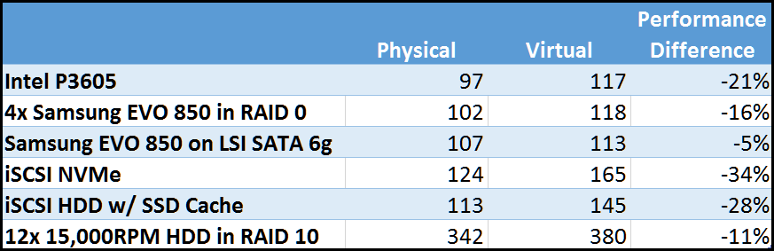
And as a graph:

CONCLUSION
In my last post, I talked about preconceived notions. In this post, I get to confirm one of those. Physical hardware is faster than virtual hardware. This shouldn’t be shocking to anyone. But, I like having a percentage and seeing the different configurations. For instance, network storage in this instance is an upgrade compared to regular hard drives. But if you are going from local SSD storage to network storage, you will end up slower on two fronts. First, you obviously lose speed going to a virtual environment. Next, you also lose speed going to the network.


 As queue depth increases, the performance differential seem to stay pretty consistent. Asynchronous performance is pulling away just a tad from the rest of the options.


